GUI user guide
The OXASL_OPTPCASL GUI is started using the command oxasl_optpcasl_gui
GUI requirements
The wxpython GUI library is required for the GUI. This is not included as a requirements of oxasl_optpcasl
since it is possible to use the optimizer solely through the command line. So, if you want to use the
GUI you will need to install wxpython, for example using one of the following:
python -m pip install wxpython
conda install wxpython
GUI errors on Mac
A common issue on Mac when a Conda environment is being used is that the GUI will fail to start with a message about requiring a ‘Framework Build’.
This is a well known issue with Conda which to date has not been fixed. To work around the problem you need to modify the wrapper script, for example using:
nano `which oxasl_optpcasl_gui`
If you are using FSL and installed oxasl_optpcasl into fslpython then change the first line to:
#!/usr/bin/env fslpythonw
Otherwise, change the first line to:
#!/usr/bin/env pythonw
This should enable to the script to run.
Overview of the GUI
The window is divided into two horizontally. The left hand pane is used to set properties of the scan protocol, assumed physiological parameters and options for the optimization process. The right hand pane displays characteristics of the selected protocol including sensitivity to ATT and CBF and illustrations of the relationship between the effective PLDs of the protocol and the PCASL kinetic curve (using the Buxton model).
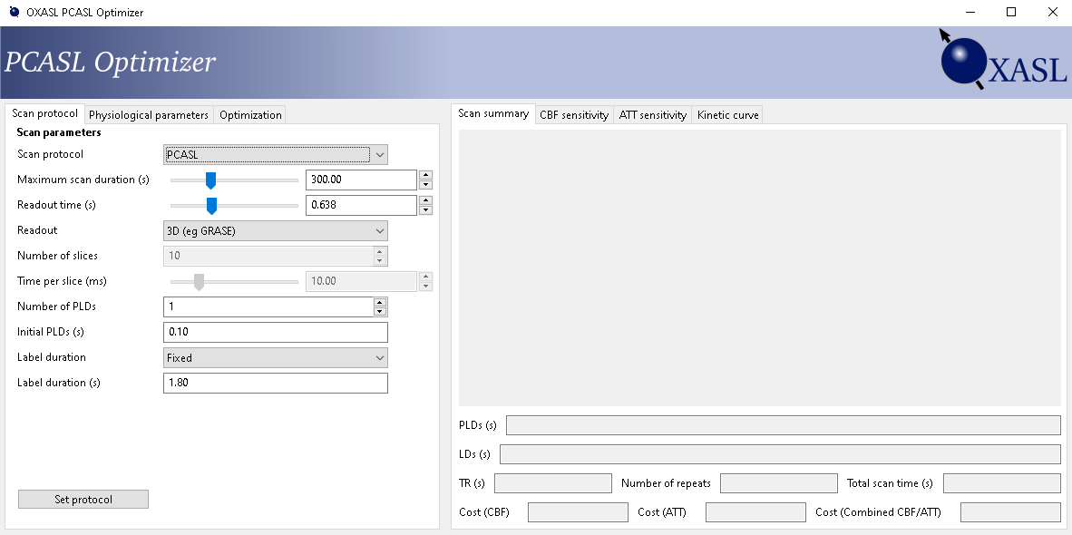
Setting the scan parameters
On the first tab we set the parameters for the scan we want to optimize. There are three basic scan protocols:
PCASL protocol
This protocol is a standard PCASL acquisition which consists of an inversion (labelling) pulse followed by a post-labelling delay (PLD) followed by readout. This cycle is then repeated but without the labelling pulse, substituting a matching control delay so the total time to readout is the same. For a single PLD this can be depicted graphically as follows:
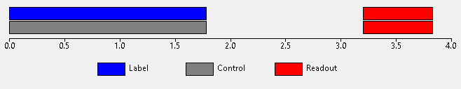
Subtraction of the labelled image from the control image is used to obtain the ASL signal.
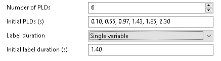
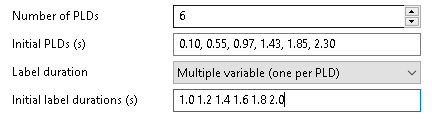
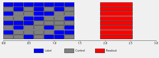
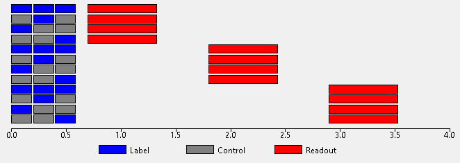
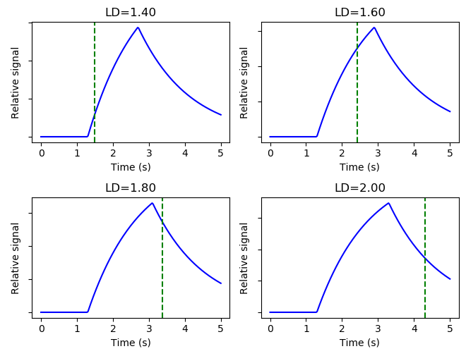
This label/control cycle can be repeated with different PLDs in order to sample the ASL kinetic curve at different points. The different PLDs may be paired with the same labelling duration (LD) or each PLD may have a different LD:
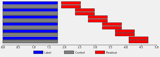
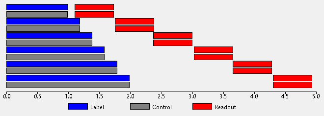
When using a PCASL protocol the initial PLDs must be specified as a space or comma separated list of values in seconds. The labelling duration may either be fixed (one value which is not optimized), single (one initial value which is optimized) or multiple (one initial value per PLD, all optimized).
Hadamard time-encoded protocol
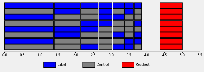
In this protocol, the labelling phase consists of a sequence of ‘sub-boli’ each of which may be either an inversion pulse or a control delay. After the full set of sub-boli there is again a post-labelling delay followed by readout. The cycle is repeated but with the label/control allocation of each sub-bolus changed for each repeat. The pattern of these label/control sub-boli across all the acquisition cycles forms a Hadamard matrix. Sizes of 4, 8 and 12 may be used (the number of sub-boli is one less than the matrix size). For example a Hadamard acquisition using a matrix of size 8 can be depicted as follows:
To obtain the ASL signal the images must be decoded by adding and subtracting each cycle. By doing this in different ways the contribution of each sub-bolus can be isolated without the need for a corresponding control cycle. Hence Hadamard encoding allows us to obtain 7 subtracted images from only 8 label/control cycles (conventional PCASL would require 14 label/control cycles to produce 7 subtracted images). We can therefore potentially extract more information in a given time.
Commonly Hadamard protocols only use a single PLD since each sub-bolus has a different effective PLD when decoded. However it is possible to repeat the entire Hadamard sequence at multiple PLDs, for example this acquisition (using a matrix size of 4 to reduce the time required):
The lengths of the Hadamard sub-boli may all be equal, however do not have to be. Once approach is to choose the length of the first sub-bolus and then choose shorter lengths for the remainder to account for T1 decay in such a way that the total signal from each sub-bolus is the same:
Alternatively, all the sub-boli durations may be specified (and optimized) independently.
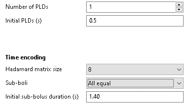
With the Hadamard protocol, the matrix size must be specified and the strategy for choosing sub-bolus durations. If these are all equal then a single initial value must be given. When using the T1 decay strategy the first sub-bolus duration is specified. When sub-bolus durations are unconstrained the initial values must be specified as space or comma separated values in seconds (one less than the matrix size):

‘Free lunch’ protocol
This is essentially a Hadamard protocol, however the first sub-bolus is fixed at a ‘long’ value typically equal to that used in single-PLD PCASL experiments. The idea here is to do a ‘normal’ single delay PCASL experiment but fill in the long PLD with additional Hadamard encoded sub-boli. The resulting images can either be analysed as a collection of 4 single-PLD label/control pairs (the remaining sub-bolus contributions cancel out in this case), or undergo Hadamard decoding to gain additional information ‘for free’. Typically we optimize the duration of the first of these sub-boli and assign the remainder using the T1 decay strategy.
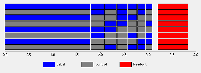
Note the similarity of this to the single-PLD experiment shown above - they are essentially the same but with the ‘spare’ PLD space filled with time-encoded labelling pulses for additional information.
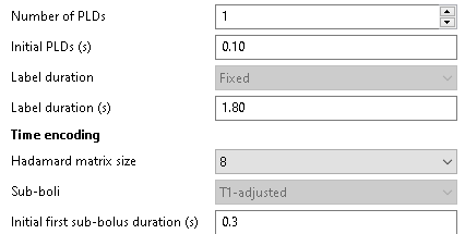
With the free-lunch protocol, a single fixed labelling duration must be given - this is not optimized. An initial value for the next sub-bolus duration must also be given, this is optimized and the remainder are chosen according to the T1 decay strategy. One or more initial PLDs is also required:
Currently it is not possible to change the strategy used to select sub-bolus durations, nor to optimize the initial ‘long’ LD. This may be added in the future.
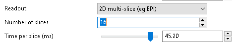
2D/3D readout
If we are using a 2D multi-slice readout, additional options for the time per slice and number of slices are enabled:
Displaying information about the protocol
Clicking the Set Protocol button loads the initial protocol design into
the output tabs on the right side of the viewing pane. Nothing has been
optimized yet, but you can view information about the protocol’s sensitivity
to ATT and CBF here.
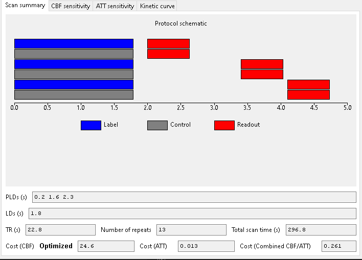
The protocol summary
This tab shows a graphical representation of the protocol together with the calculated cost values for measuring CBF, ATT and combined CBF/ATT cost. The optimization process will seek to modify the PLDs/LDs of the protocol to minimise one of these values.
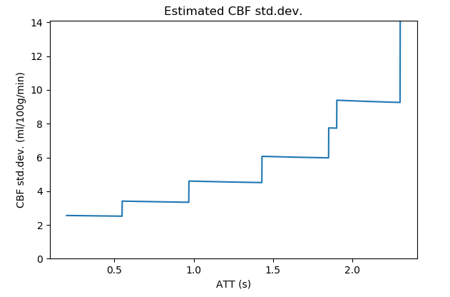
Sensitivity to CBF
This plot shows the sensitivity of the protocol to CBF at a range of arterial transit times. For example, in the plot below we can see that this protocol becomes less sensitive to CBF at longer ATTs. Sensitivity plots often have ‘steps’ in them which generally correspond to the PLDs.
Kinetic curve
This tab shows an illustration of the simple Buxton model of the ASL signal with the protocol PLDs displayed as vertical dashed lines. Note that for time encoded (Hadamard) protocols, the PLDs shown are the effective PLDs for each sub-bolus after decoding. The slider at the bottom can be used to view the kinetic curve at different ATTs.
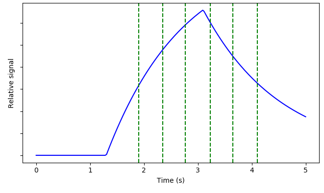
In protocols with multiple labelling durations a different kinetic curve is plotted for each.
Optimization configuration
On the ‘Optimization’ tab, we can control the optimization parameters. This includes the prior distribution of ATT and the search limits for PLDs. However the most likely setting to change here is whether we want to optimize for CBF, ATT or both.
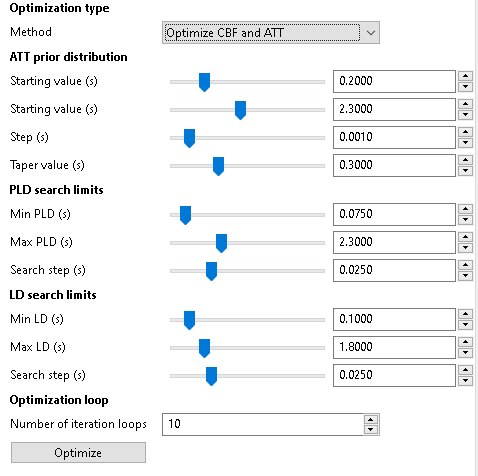
The optimization works by modifying one parameter (PLD or LD) at a time and sometimes can reach different results depending on what order it chooses to optimize each parameter. To make the results more robust it is common to repeat the optimization cycle multiple times (the order is chosen randomly each time) and choose the outcome with the lowest cost. When optimizing a small number of parameters (e.g. a single LD and PLD) multiple runs may be unnecessary, however when multiple PLDs and LDs are to be optimized it may be helpful to run the optimization a large number of times - of course this may take a while!
Running the optimization
Click the Run Optimization button to start - it may take a few seconds for
a simple optimization with a single repeat, or many minutes for cases with
many parameters or where multiple optimization loops have been specified. Fine
PLD/LD search spacings and large ATT prior distributions may also increase the
time required for optimization.
After optimization, the output pane will be updated to show the optimized
protocol. The label Optimized will be shown beside the cost measure that
has been optimized.
Sample output
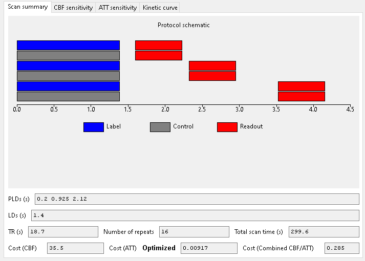
This is the output of an optimized multi-PLD PCASL experiment with 3 PLDs and a single optimized labelling duration.
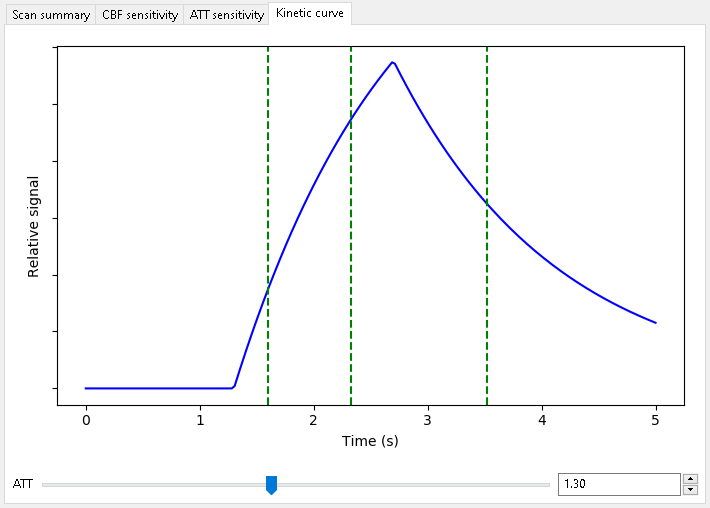
When optimizing for CBF alone, we get the following scan:
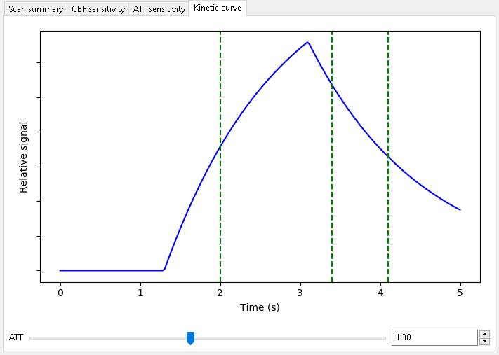
Note that two of the three PLDs are in the decay part of the curve for most ATTs (this plot was obtained for ATT=1.3). This is good for estimating CBF as the whole bolus has usually arrived by this point.
When optimizing for ATT alone, we get the following scan:
As expected, when optimizing for ATT measurements, shorter PLDs are preferred to sample the inflow of the bolus.
When optimizing for CBF and ATT we obtain the following:
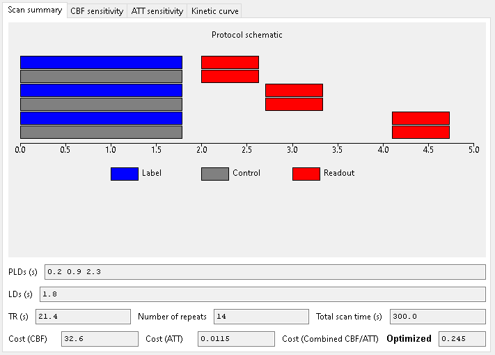
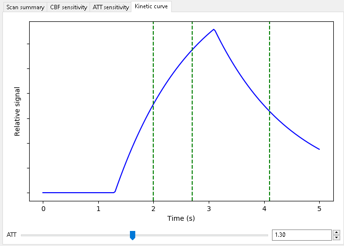
The combined optimization is in between the CBF and ATT-only extremes with longer PLDs than the ATT-only optimization but shorter than the CBF-only case.
Physiological parameters
The Physiological parameters tab allows control of the assumed values of parameters used in the kinetic model (and hence affecting the cost function and optimization).
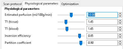
The estimated perfusion is a fixed value used to calculate the effective T1 of labelled blood. Modification of this value should not have a significant effect on the cost or optimization, however.